01 | Rhythm and Time | 01 | Intro to Rhythm Trees

Trees¶

A tree is a graph where any two nodes are connected by exactly one path. Each node can have multiple children but only one parent, except for the root node, which has no parent. Nodes with no children are called leaf nodes.

Ok, but what does that mean, exactly? Let’s visualize it.

Here is a binary tree (each node has at most 2 children):

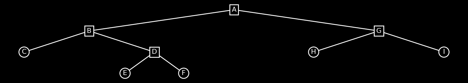
Leaf nodes are depicted with circles. A is the root—it has no parent. Every other node has either two children or no children.

Nodes (other than the root) that do have children are called inner nodes. Nodes that have a parent, but have no children are called leaf nodes.

Trees do not have to be binary. A k-ary tree allows nodes to have up to k children:

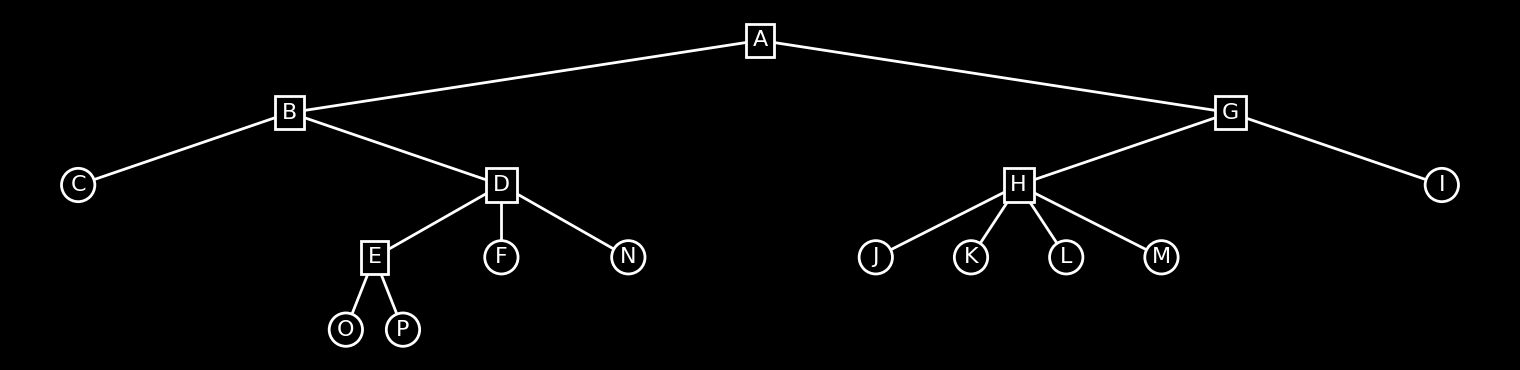
This is a 4-tree: node H has 4 children, the maximum. Other nodes use fewer. Not every node needs the full k-number of children.

The depth of a tree is the distance from the root to the furthest leaf. The tree above has depth 4: nodes O and P are 4 levels from root A.

Rhythm Trees¶

A Rhythm Tree (RT) describes hierarchical rhythmic structure as a k-ary tree.

As we saw in the Principles of Proportion notebook, the durations in an RT are relative proportions of a parent container — not absolute values. No matter how we subdivide, the proportions always account for the whole.

With that foundation in place, let’s explore what makes Rhythm Trees truly powerful: nesting.

Nesting and Recursion¶

So far these have all been flat lists. The tree structure becomes interesting when we start nesting subdivisions.

Let’s subdivide the first element of (4 2 1 1) into three equal parts. So, we’ll go from this..

...to this...

The first subdivision now has three children. Let’s check out the resultant rhythmic ratios:

More ratios (because we have more subdivisions), but they still sum to 1.

Instead of this tree view, it may become clearer to look at the structure like “containers”:

Each level represents a level in the tree and each block represents a node. Children of a node are blocks placed directly below. The thin line at the bottom shows the resultant ratios—i.e., the rhythm.

Compare this representation to the tree representation. Do you see how both are representations of the same thing?

Let’s add another level of subdivisions...

...and the same thing, but represented as containers...

Even more subdivisions, still sums to 1.

Question: Given a tree, how can we tell how many “notes” we’ll have in our rhythm?

Answer: Count the number of leaf nodes. Go back and look at the above RTs, count the number of leaves and compare to the number of note events in the rhythm. It’s always the same.

The (D S) Formalism¶

Let’s take a moment to formally define a Rhythm Tree (RT).

An RT is defined as a pair (D S) where:

• D is a positive, non-zero integer representing a duration.

• S is a list of proportional subdivisions of D.

Each element of S is either a non-zero integer or another (D S) pair. This means RTs can be nested: a subdivision can be subdivided, which can also be subdivided, and so on...

That is to say, RTs are a recursive structure.

Group Notation¶

How does the last RT we made look in this (D S) format? Like this: ((1 ((4 (1 1 (1 (1 1)))) 2 1 1)))

Ok, if you’re confused by that, don’t worry. This notation is a bit difficult to digest at first. So, let’s break down how we arrived at this...

We started with some block of time, duration 1. We then subdivided it into four proportions. That gave us this:

(1 (4 2 1 1))

Where D = 1, and S = (4 2 1 1). So, (D S) = (1 (4 2 1 1)).

We then subdivided the first element of S, 4. Recall, each element of S is either a non-zero integer or another (D S) pair. So, that gave us:

(1 ((4 (1 1 1)) 2 1 1))

We then subdivided the last subdivision of the 4 segment by splitting 1 into (1 (1 1)), giving us:

((1 ((4 (1 1 (1 (1 1)))) 2 1 1)))

This is what’s called group notation. It comes from the LISP programming language. The name “LISP” is an abbreviation for “list processing”. Although, a common joke is that it really stands for Lost In Stupid Parenthesis.

There’s a certain degree of truth in that joke... it’s not exactly the most intuitive notation if you’re experiencing it for the first time. This is one of the reasons we conceptualize and visualize RTs as tree graphs, or as a stack of “containers”. The group notation is actually encoding this tree/container formalism, it’s just not immediately clear if you’re not used to it.

When we create an RT in Klotho, we can always access its group notation like this:

We can also access additional information about the RT like this:

Rests in Trees¶

Recall from before that negative numbers represent rests — silent segments that take up the same proportional share as their positive counterparts. This works exactly the same way in nested trees.

But there’s an additional nuance with nesting: what happens when the D-part of a sub-tree is negative? Let’s recall the formal definition. An RT is a pair (D S) where D is a positive, non-zero integer. Values inside S must simply be non-zero — they can be negative (rests) or positive (sounding). But D must be positive.

...or must it? What happens if we break the rule?

Let’s make an RT with a rest:

The rest is greyed out. The proportion is the same; only the sign changed.

More rests:

What happens if we make the D-part of an RT negative? This makes the entire subtree a rest, including all its descendants:

The third segment’s D is -1. Its children still define the internal proportions, but the whole subtree is silent.

This isn’t exactly wrong, but it’s not the best notational practice. The above rhythm would be better notated like this:

Do you see why? The resultant rhythm is exactly the same (or, rather, sounds exactly the same), but the notation is a clearer representation of what is happening: we rest for a 1/4-note (because four 1/16s equals 1/4).

The prior version is an example of something that is syntactically correct, by semantically confusing.

Meas & Span¶

Meas¶

So far, we’ve been setting our parent container to 1. This represents the total duration of the RT, which is why the sum the resultant ratios as been 1. In group notation, this is the outermost value of D. We refer to this as the meas of the RT.

Now, keeping all the internal proportions exactly the same, let’s adjust the meas a few times and expand or contract the total duration of the rhythm:

So, between each example, what changed and what stayed the same?

We can think of the meas as a means of fine-tuning, or scaling, the overall duration of our rhythm.

So, is the meas just another way of saying time signature?¶

No.

Yes...

...kinda...

...but not exactly.

Let’s examine these nuances.

You can think of meas as a time signature — if you want to. For example, an RT with meas='4/4' fits within a standard 4/4 measure. But the RT formalism doesn’t require you to think of it that way.

Consider: you can write an RT with meas='4/4' whose internal subdivisions completely disregard any notion of meter. In that case, meas is just a container of a certain size — 4/4 = 1/1, meaning “this rhythm fits within the duration of 4 quarter-notes, or one whole note.” The subdivisions inside might have nothing to do with beats, downbeats, or metric regularity.

Here’s an example that clearly respects 4/4 meter — four quarter-note beats, each subdivided into binary divisions — and another that does not:

It’s a matter of perspective and intent.

And it doesn’t necessarily imply any particular notation either. Imagine 4 RTs in sequence, each with a meas of 1/4. Is that four measures of 1/4 time? Perfectly valid, but maybe not the most readable notation.

Or are you just thinking of four “free” quarter-notes, each with their own internal subdivisions, with no barlines between them at all? You could notate it either way — or consolidate it into a single measure of 4/4. The meas simply defines the size of the outer-most container at an abstract level; what that size means musically, and how it’s expressed in notation, is up to you.

What’s up with these weird meas values like 2/3 and 6/5? Those don’t look like time signatures I’ve seen before...¶

Let’s take a step back and think about what a time signature actually is.

It all starts with the whole note. If we slice a whole note into 4 equally proportioned slices, we get 4 quarter notes (1/4 notes). Slice it into 8 equally proportioned slices and we get 8 eighth notes (1/8 notes). 2 slices gives us 2 half notes (1/2 notes), 16 gives us 16 sixteenth notes (1/16 notes), and so on. The denominator of the note fraction tells us how many of that note fit in a whole note.

A time signature like 4/4 says: a unit of time consisting of 4 quarter-notes. We can read this as both a description of the unit’s total duration (4/4 = one whole note) and as the primary “branches” that we can further subdivide.

If n * (1/n) = 1, the time signature spans exactly one whole note — 4/4, 8/8, 16/16, etc. But this isn’t always the case. 3/4 is a unit of time spanning 3 quarter-notes — 3/4 of a whole note (so, smaller than a whole note). 5/4 is a unit of time spanning 5 quarter-notes — 5/4 of a whole note (so, larger than a whole note).

Again, both a duration descriptor and an indicator of the top-level branches (3 quarter-notes, each of which can be further subdivided).

Os, so then what about these non-powers-of-two denominators? If we slice a whole note into 5 equally proportioned slices, we get 5 “fifth-notes” (1/5 notes). Three slices give us 3 “third-notes” (1/3 notes). These are perfectly valid note values — they’re just not standard in traditional notation.

These so-called “irrational” time signatures follow the exact same logic. A meas of 3/5 says: a unit that spans 3/5 of a whole note, consisting of 3 “fifth-notes.” A meas of 7/3 says: a unit that’s 7/3 of a whole note (longer than a whole note), where the main beats are delimited by 7 “third-notes.”

Worth noting: there’s actually nothing irrational about these time signatures in the mathematical sense — they are all quite literally rational numbers, by definition. The name “irrational” is just a convention from music notation associated with the New Complexity that stuck, referring to time signatures with non-power-of-two denominators. A more accurate label might be “non-binary,” but here we are.

It’s also worth reiterating that we don’t need to think of these as time signatures in the conventional sense either—we’re just describing the size of the outer-most container of our rhythm.

Does a meas of 2/3 mean a measure with a time signature of 2/3 or does it just mean some temporal unit with a duration of two-thirds of a whole note? It’s up to you.

You can think of it as generally as an overall duration, or you can compose the contained rhythm to adhere to the metric implications of the meas if you so choose.

This is one reason we use the term meas in RT syntax instead of time signature. We want to capture this nuance.

Span¶

Let’s say we’ve decided on a meas. We can multiply it n-number of times using the span parameter. If the meas is the shape of our rhythmic container, the span is like saying, “how many of these meas-sized units does the rhythm span?”

In the early examples, we always set both span and meas to 1, therefore our rhythmic ratios always summed to 1. If, e.g., we set meas to 5/4 and span to 3, the total duration of our rhythm would be 3 * 5/4 = 15/4.

We can think of this like saying the rhythm is contained within one measure of 15/4 or spead across 3 measure of 5/4. Or, more generally, that the rhythm spans a duration of 15 1/4-notes.

Notice that we haven’t looped our rhythm span-number of times. We’ve just adjusted the total size of the outermost container. The total duration of an RT (which is to say, the sum of its rhythmic ratios) is always span * meas.

But what if we want to actually loop our rhythm n-number of times? How do we do that? We’ll answer that in the coming notebooks.