from klotho import Tree, RhythmTree as RT, plot, play
from fractions import Fraction
from klotho.thetos import JsInstrument as JsInst, CompositionalUnit as UC
from klotho.chronos import TemporalUnitSequence as UTS, TemporalBlock as BT
from klotho.topos import Pattern, PartitionSet as PS
from klotho.tonos import Scale, Contour
import numpy as np# Chronostasis
tempus = '10/16'
beat = '1/16'
bpm = 140
n_bars = 4
S1 = ((3, (1,)*4), (4, (1,)*6), (3, (1,)*4))
S2 = ((5, (1,)*5),)*2
inst_pat_1 = Pattern([JsInst.HatClosed(), [JsInst.HatClosed(), [[JsInst.TomHigh(), JsInst.TomMid()], [JsInst.HatOpen(), [JsInst.Ride(decay=0.2), JsInst.HatClosed()]]]]])
uc1 = UC(tempus=tempus, prolatio=S1, beat=beat, bpm=bpm)
uts1 = uc1.repeat(n_bars)
for unit in uts1:
unit.set_instrument(unit.leaf_nodes, inst_pat_1)
unit.set_pfields(unit.leaf_nodes, vel=lambda: np.random.uniform(0.001, 0.25))
inst_pat_2 = Pattern([[[JsInst.Kick("kick_punchy", punch=16), JsInst.Kick("kick_pitchy", pitchDecay=0.05, decay=0.9)], JsInst.Snare()], JsInst.Kick()])
uc2 = UC(tempus=tempus, prolatio=S2, beat=beat, bpm=bpm)
uts2 = uc2.repeat(n_bars)
for unit in uts2:
unit.set_instrument(unit.leaf_nodes, inst_pat_2)
unit.set_pfields(unit.leaf_nodes, vel=lambda: np.random.uniform(0.75, 0.9))
play(BT([uts1, uts2]))...or like this?
# Entertain Me

tempus = '36/16'
beat = '1/8'
bpm = 184
n_bars = 2

scale = Scale.phrygian().root('B3')

S1 = ((20, ((5, (1,)*5),)*4), (15, ((3, (1,)*3),)*5))

uc_mel = UC(tempus=tempus, prolatio=S1, beat=beat, bpm=bpm, inst=JsInst.Kalimba())
limbs = uc_mel.at_depth(1)
uc_mel.set_mfields(limbs[0], idx=0, drct=1, offset=0)
uc_mel.set_mfields(limbs[1], idx=len(scale), drct=-1, offset=0)
uc_mel.set_mfields(list(uc_mel.successors(limbs[-1])), offset=lambda c: c.total - c.index)

for branch in uc_mel.at_depth(2):
    uc_mel.set_pfields(
        uc_mel.subtree_leaves(branch),
        freq=lambda c: scale[c.params['offset'] + c.params['idx'] + c.params['drct'] * c.index].freq
    )

uc_ds = UC(tempus=tempus, prolatio=S1, beat=beat, bpm=bpm)
uc_ds.set_instrument(uc_ds.subtree_leaves(limbs[0]), Pattern([[JsInst.Kick(), JsInst.Snare()], JsInst.HatClosed()]))
uc_ds.set_instrument(uc_ds.subtree_leaves(limbs[-1]), lambda c: JsInst.HatOpen(vel=0.1) if c.index % 2 == 0 else JsInst.HatClosed())

uc_bs = UC(tempus=tempus, prolatio=S1, beat=beat, bpm=bpm, inst=JsInst.Bassy(freq=scale[-len(scale)*2].freq, vel=0.2))
bs_pat = Pattern([0, 0, [1, [3, [4, -3]]]])
uc_bs.make_rest(limbs[-1])
seq_bs = uc_bs.repeat(n_bars)
for unit in seq_bs:
    unit.set_pfields(unit.leaf_nodes, freq=lambda: scale[next(bs_pat) - len(scale)*2].freq)

play(BT([uc_mel.repeat(n_bars), uc_ds.repeat(n_bars), seq_bs]))...or like this?
# Polyriddim

S1 = ((1, ((6, (1,)*7), (8, (1,)*11))), (1, ((6, ((3, (1,)*4), 1, (2, (1,)*3))), (8, ((3, (1,)*4), (3, (1,)*4), (5, (1,)*5))))), (1, ((6, (2, (3, (1,)*4), (2, (1,)*4))), (8, ((2, (1,)*3), (2, (1,)*4), (2, (1,)*5), (2, (1,)*5))))), (1, ((6, ((2, (1,)*3), (2, (1,)*3), (2, (1,)*3))), (8, (5, (6, (1,)*11))))))
S2 = ((7, ((3, (1,)*3), (4, (1,)*4))),)*4

tempus = '28/16'
beat = '1/16'
bpm = 122.5

inst1_pat = Pattern([
    [JsInst.Kick(), [
        [JsInst.Kick("kick_punch", punch=9, click=0.6), JsInst.Snare("snare_body", body=0.8)], JsInst.TomMid()]],
    [JsInst.Kick("kick_click", click=0.8), [
        [JsInst.Snare(), JsInst.TomHigh(punch=8, decay=0.9)], JsInst.TomLow()]]
])

n_bars = 2

uc1 = UC(tempus=tempus, prolatio=S1, beat=beat, bpm=bpm)
uts1 = uc1.repeat(n_bars)
for unit in uts1:
    unit.sparsify(0.33)
    unit.set_instrument(unit.leaf_nodes, inst1_pat)
    unit.set_pfields(unit.leaf_nodes, vel=lambda: np.random.uniform(0.25, 0.85))

uc2 = UC(tempus=tempus, prolatio=S2, beat=beat, bpm=bpm)
uts2 = uc2.repeat(n_bars)
for unit in uts2:
    for branch in unit.at_depth(2):
        unit.set_instrument(branch, JsInst.HatClosed())
        unit.set_instrument(unit.successors(branch)[-1], JsInst.HatOpen())
        unit.set_pfields(unit.subtree_leaves(branch), vel=lambda: np.random.uniform(0.05, 0.25))

scale = Scale.locrian().root('Eb2')
scl_pat = Pattern([[0, -1, [0, -3]], [1, [3, 4]]])
uc3 = UC(tempus=tempus, prolatio=S1, beat=beat, bpm=bpm, inst=JsInst.Bassy())
uts3 = uc3.repeat(n_bars)
for unit in uts3:
    unit.sparsify(0.67)
    unit.set_pfields(unit.leaf_nodes, freq=lambda: scale[next(scl_pat)].freq, vel=lambda: np.random.uniform(0.1, 0.5))

play(BT([uts1, uts2, uts3]))Trees
A tree is a graph where any two nodes are connected by exactly one path. Each node can have multiple children but only one parent, except for the root node, which has no parent. Nodes with no children are called leaf nodes.
Here is a binary tree (each node has at most 2 children):
plot(Tree('A', (('B', ('C', ('D', ('E', 'F')))), ('G', ('H', 'I')))), figsize=(15, 2.5))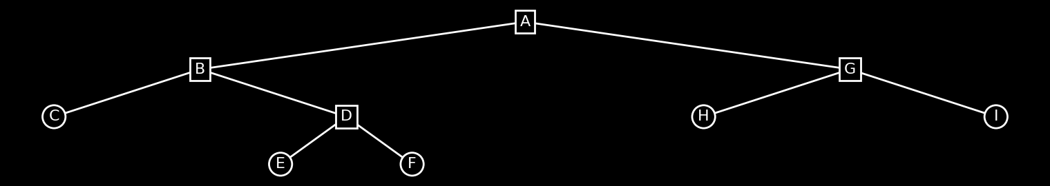
Leaf nodes are depicted with circles. A is the root.
Trees do not have to be binary. A k-ary tree allows nodes to have up to k children:
plot(Tree('A', (('B', ('C', ('D', (('E', ('O', 'P')), 'F', 'N')))), ('G', (('H', ('J', 'K', 'L', 'M')), 'I')))), figsize=(15, 3.5))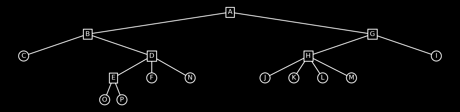
This is a 4-tree: node H has 4 children, the maximum. Other nodes use fewer. Not every node needs the full k.
The depth of a tree is the distance from the root to the furthest leaf. The tree above has depth 4: nodes O and P are 4 levels from root A.
Rhythm Trees
A Rhythm Tree (RT) describes hierarchical rhythmic structure as a k-ary tree.
As we saw in the Principles of Proportion notebook, the durations in an RT are relative proportions of a parent container — not absolute values. No matter how we subdivide, the proportions always account for the whole.
With that foundation in place, let’s explore what makes Rhythm Trees truly powerful: nesting.
Nesting and Recursion
So far these have all been flat lists. The tree structure becomes interesting when we start nesting subdivisions.
Let’s subdivide the first element of (4 2 1 1) into three equal parts. So, we’ll go from this..
rt = RT(subdivisions=(4, 2, 1, 1))
plot(rt, layout='tree', animate=True, beat='1/4', bpm=120)...to this...
# plot(Tree(1, ((4, (1, 1, 1)), 2, 1, 1)), figsize=(20, 3))
rt = RT(subdivisions=((4, (1, 1, 1)), 2, 1, 1))
plot(rt, layout='tree', animate=True, beat='1/4', bpm=120)The first subdivision now has three children. Let’s check out the resultant rhythmic ratios:
print('Durations:', *[str(d) for d in rt.durations])
print('Sum:      ', sum(rt.durations))
Durations: 1/6 1/6 1/6 1/4 1/8 1/8
Sum: 1
More ratios (because we have more subdivisions), but they still sum to 1.
Instead of this tree view, it may become clearer to look at the structure like “containers”:
plot(rt, layout='containers', animate=True, beat='1/4', bpm=120)Each level represents a level in the tree and each block represents a node. Children of a node are blocks placed directly below. The thin line at the bottom shows the resultant ratios—i.e., the rhythm.
Compare this representation to the tree representation. Do you see how both are representations of the same thing?
Let’s add another level of subdivisions...
rt = RT(subdivisions=((4, (1, 1, (1, (1, 1)))), 2, 1, 1))
plot(rt, layout='tree', figsize=(11, 2.5), animate=True, beat='1/4', bpm=120)...and the same thing, but represented as containers...
plot(rt, layout='containers', animate=True, beat='1/4', bpm=120)print('Durations:', *[str(d) for d in rt.durations])
print('Sum: ', sum(rt.durations))Durations: 1/6 1/6 1/12 1/12 1/4 1/8 1/8
Sum: 1
Even more subdivisions, still sums to 1.
Question: Given a tree, how can we tell how many “notes” we’ll have in our rhythm?
Answer: Count the number of leaf nodes. Go back and look at the above RTs, count the number of leaves and compare to the number of note events in the rhythm. It’s always the same.
The (D S) Formalism
Let’s take a moment to formally define a Rhythm Tree (RT).
An RT is defined as a pair (D S) where:
Dis a positive, non-zero integer representing a duration.Sis a list of proportional subdivisions ofD.
Each element of S is either a non-zero integer or another (D S) pair. This means RTs can be nested: a subdivision can be subdivided, which can also be subdivided, and so on...
That is to say, RTs are a recursive structure.
Group Notation
How does the last RT we made look in this (D S) format? Like this: ((1 ((4 (1 1 (1 (1 1)))) 2 1 1)))
Ok, if you’re confused by that, don’t worry. This notation is a bit difficult to digest at first. So, let’s break down how we arrived at this...
We started with some block of time, duration 1. We then subdivided it into four proportions. That gave us this:
(1 (4 2 1 1))
Where D = 1, and S = (4 2 1 1). So, (D S) = (1 (4 2 1 1)).
We then subdivided the first element of S, 4. Recall, each element of S is either a non-zero integer or another (D S) pair. So, that gave us:
(1 ((4 (1 1 1)) 2 1 1))
We then subdivided the last subdivision of the 4 segment by splitting 1 into (1 (1 1)), giving us:
((1 ((4 (1 1 (1 (1 1)))) 2 1 1)))
This is what’s called group notation. It comes from the LISP programming language. The name “LISP” is an abbreviation for “list processing”. Although, a common joke is that it really stands for Lost In Stupid Parenthesis.
There’s a certain degree of truth in that joke... it’s not exactly the easiest notation to read. This is one of the reasons we conceptualize and visualize RTs as tree graphs, or as a stack of “containers”. This is actually what the group notation is encoding, it’s just not immediately clear if you’re not used to it.
When we create an RT in Klotho, we can always access its group notation like this:
rt = RT(meas=1, subdivisions=((4, (1, 1, (1, (1, 1)))), 2, 1, 1))
print(rt.group)
Group((1 ((4 (1 1 (1 (1 1)))) 2 1 1)))
We can also access additional information about the RT like this:
print(rt.info)--------------------------------------------------
span: 1 | meas: 1/1 | type: None | depth: 3 | k: 4
--------------------------------------------------
Subdivs: ((4 (1 1 (1 (1 1)))) 2 1 1)
--------------------------------------------------
Onsets: 0 1/6 1/3 5/12 1/2 3/4 7/8
Durations: 1/6 1/6 1/12 1/12 1/4 1/8 1/8
--------------------------------------------------
Rests
In music, we don’t always play every note. Silence is as important as sound. We call these placements of silence, rests.
In RT syntax, these are notated as negative numbers. Let’s recall the formal definition of an RT:
An RT is defined as a pair (D S) where:
Dis a positive, non-zero integer representing a duration.Sis a list of proportional subdivisions ofD.
Each element of S is either a non-zero integer or another (D S) pair.
Ah ha, do you see it? Values for D must be positive and non-zero. Values inside S must simply be non-zero. We have very deliberately not said they must be positive.
Let’s make an RT with a rest:
S = (1, (1, (1, 1)), (1, (1, 1, -1, 1)), (1, (1, 3)))
rt = RT(subdivisions=S)
plot(rt, layout='containers', animate=True, beat='1/4', bpm=84)The rest is greyed out. The proportion is the same; only the sign changed.
More rests:
S = (1, (1, (1, (1, (-1, 1)))), (1, (1, 1, -1, 1)), (1, (-1, 2, 1)))
rt = RT(subdivisions=S)
plot(rt, layout='containers', figsize=(11, 2), animate=True, beat='1/4', bpm=84)What happens if we make the D-part of an RT negative? This makes the entire subtree a rest, including all its descendants:
S = (1, (1, (1, 1)), (-1, (1, 1, 1, 1)), (1, (1, 3)))
rt = RT(subdivisions=S)
plot(rt, layout='containers', animate=True, beat='1/4', bpm=120)The third segment’s D is -1. Its children still define the internal proportions, but the whole subtree is silent.
This isn’t exactly wrong, but it’s not the best notational practice. The above rhythm would be better notated like this:
S = (1, (1, (1, 1)), -1, (1, (1, 3)))
rt = RT(subdivisions=S)
plot(rt, layout='containers', animate=True, beat='1/4', bpm=120)Do you see why? The resultant rhythm is exactly the same (or, rather, sounds exactly the same), but the notation is a clearer representation of what is happening: we rest for a 1/4-note.
The prior version is an example of something that is syntactically correct, by semantically confusing.
Meas & Span
Meas
So far, we’ve been setting our parent container to 1. This represents the total duration of the RT, which is why the sum the resultant ratios as been 1. In group notation, this is the outermost value of D. We refer to this as the meas of the RT.
S = ((3, (1, (2, (-1, 1, 1)))), (5, (1, -2, (1, (1, 1)), 1)), (3, (-1, 1, 1)), (5, (2, 1)))
rt = RT(meas=1, subdivisions=S)
print(rt.info)
plot(rt, layout='tree', figsize=(11, 2), animate=True, beat='1/4', bpm=64)
--------------------------------------------------------------------------------------------------
span: 1 | meas: 1/1 | type: None | depth: 3 | k: 4
--------------------------------------------------------------------------------------------------
Subdivs: ((3 (1 (2 (-1 1 1)))) (5 (1 -2 (1 (1 1)) 1)) (3 (-1 1 1)) (5 (2 1)))
--------------------------------------------------------------------------------------------------
Onsets: 0 1/16 5/48 7/48 3/16 1/4 3/8 13/32 7/16 1/2 9/16 5/8 11/16 43/48
Durations: 1/16 -1/24 1/24 1/24 1/16 -1/8 1/32 1/32 1/16 -1/16 1/16 1/16 5/24 5/48
--------------------------------------------------------------------------------------------------
Now, keeping all the internal proportions exactly the same, let’s adjust the meas a few times and expand or contract the total duration of the rhythm:
S = ((3, (1, (2, (-1, 1, 1)))), (5, (1, -2, (1, (1, 1)), 1)), (3, (-1, 1, 1)), (5, (2, 1)))

for meas in ['3/4', '6/5', '2/3', '7/2']:
    rt = RT(meas=meas, subdivisions=S)
    print(f'meas = {meas}')
    play(rt, beat='1/4', bpm=64)
    print('-'*13)
meas = 3/4
-------------
meas = 6/5
-------------
meas = 2/3
-------------
meas = 7/2
-------------
So, between each example, what changed and what stayed the same?
We can think of the meas as a means of fine-tuning the overall length of our rhythm.
So, is the meas just another way of saying time signature?
Yes... kinda. But not exactly. Here’s why:
What about when the meas denominator is NOT a power of 2?
This is a good question.
Span
Let’s say we’ve decided on a meas. We can multiply it n-number of times using the span parameter. If the meas is the shape of our rhythmic container, the span is like saying, “how many of these meas-sized units does the rhythm span?”
In the early examples, we always set both span and meas to 1, therefore our rhythmic ratios always summed to 1. If, e.g., we set meas to 5/4 and span to 3, the total duration of our rhythm would be 3 * 5/4 = 15/4.
We can think of this like saying the rhythm is contained within one measure of 15/4 or spead across 3 measure of 5/4. Or, more generally, that the rhythm spans a duration of 15 1/4-notes.
for span in [1, 2, 3]:
    meas = '5/4'
    rt = RT(span=span, meas=meas, subdivisions=((1, (1, 1, 1)), 1, 1, (1, (1, 1)), 1))
    print(f"meas = {meas}, span = {span} -> {span} * {meas} = {str(span * Fraction(meas))}")
    print('Ratios:', *[str(d) for d in rt.durations])
    # plot(rt, layout='containers', figsize=(20, 2))
    play(rt, beat='1/4', bpm=154)
    print()
print('...and so on...')
meas = 5/4, span = 1 -> 1 * 5/4 = 5/4
Ratios: 1/12 1/12 1/12 1/4 1/4 1/8 1/8 1/4
meas = 5/4, span = 2 -> 2 * 5/4 = 5/2
Ratios: 1/6 1/6 1/6 1/2 1/2 1/4 1/4 1/2
meas = 5/4, span = 3 -> 3 * 5/4 = 15/4
Ratios: 1/4 1/4 1/4 3/4 3/4 3/8 3/8 3/4
...and so on...
Notice that we haven’t looped our rhythm span-number of times. We’ve just adjusted the total size of the outermost container. The total duration of an RT (which is to say, the sum of its rhythmic ratios) is always span * meas.
But what if we want to actually loop our rhythm n-number of times? How do we do that? We’ll answer that in the coming notebooks.